共享内存
目录
共享内存
异步调度器接受任何 concurrent.futures.Executor 实例。这包括 Python 标准库中定义的 ThreadPoolExecutor 和 ProcessPoolExecutor 实例,以及来自第三方库的任何其他子类。Dask 还定义了自己的 SynchronousExecutor,它只在主线程上运行函数(对调试很有用)。
完整的 Dask get 函数分别存在于 dask.threaded.get、dask.multiprocessing.get 和 dask.get 中。
策略
异步调度器维护索引数据结构,这些结构显示哪些任务依赖于哪些数据,哪些数据可用,哪些数据在等待哪些任务完成后才能释放,以及哪些任务当前正在运行。相对于总任务数和可用任务数,它可以在常数时间内更新这些信息。这些索引结构使得 Dask 异步调度器能够在单台机器上扩展到非常多的任务。
为了保持较小的内存占用,我们选择将就绪任务保存在后进先出栈中,以便最近可用的任务获得优先权。这鼓励在开始新链之前完成相关任务链。这也可以在常数时间内查询。
性能
tl;dr 线程调度器开销大致如下
每个任务 200 微秒的开销
10 微秒的启动时间(如果您每次都希望创建一个新的 ThreadPoolExecutor)
随任务数量的常数扩展
随每个任务依赖数量的线性扩展
调度器会引入开销。这种开销有效地限制了我们并行处理的粒度。下面我们将测量异步调度器在使用不同的 apply 函数(线程、同步、多进程)以及在不同负载类型(易并行、密集通信)下的开销。
我们可以做的最快/最简单的测试是使用 IPython 的 timeit magic 函数
In [1]: import dask.array as da

In [2]: x = da.ones(1000, chunks=(2,)).sum()

In [3]: len(x.dask)
Out[3]: 1168

In [4]: %timeit x.compute()
80.9 ms +- 387 us per loop (mean +- std. dev. of 7 runs, 10 loops each)
因此每个任务大约需要 ~90 微秒。其中大约 100 毫秒来自开销
In [5]: x = da.ones(1000, chunks=(1000,)).sum()

In [6]: %timeit x.compute()
1.06 ms +- 3.65 us per loop (mean +- std. dev. of 7 runs, 1,000 loops each)
每次启动 ThreadPoolExecutor 都会有一些开销。这可以通过使用全局或上下文线程池来缓解。
>>> from concurrent.futures import ThreadPoolExecutor
>>> pool = ThreadPoolExecutor()
>>> dask.config.set(pool=pool)  # set global ThreadPoolExecutor

or

>>> with dask.config.set(pool=pool)  # use ThreadPoolExecutor throughout with block
...     ...
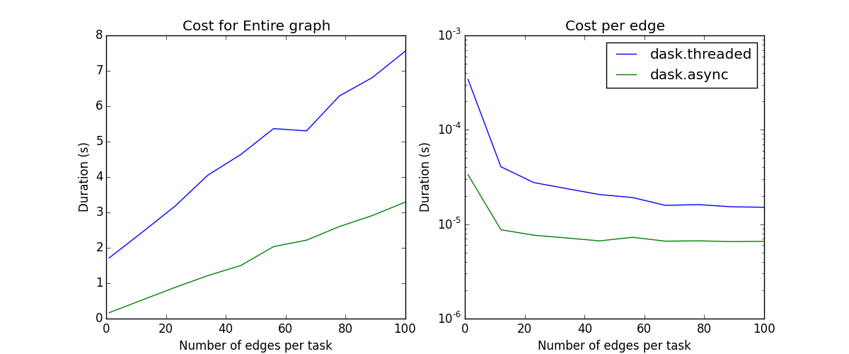
现在我们测量任务数量的扩展和图密度的扩展


已知限制
共享内存调度器有一些显著的限制
它在单台机器上工作
线程调度器受 Python 代码的 GIL 限制,因此如果您的操作是纯 Python 函数,您不应该期望多核加速
多进程调度器必须在 Worker 之间序列化函数,这可能会失败
多进程调度器必须在 Worker 和中心进程之间序列化数据,这可能会很昂贵
多进程调度器无法直接在 Worker 进程之间传输数据;所有数据都通过主进程路由。