Dask 十分种入门

Dask 十分种入门¶

这是为新用户准备的 Dask 简短概览。文档的其余部分包含更多信息。

Dask overview. Dask is composed of three parts: collections, task graphs, and schedulers.

高级集合用于生成任务图，任务图可以由调度程序在单机或集群上执行。¶

我们通常按如下方式导入 Dask

>>> import numpy as np
>>> import pandas as pd

>>> import dask.dataframe as dd
>>> import dask.array as da
>>> import dask.bag as db

根据您处理的数据类型，您可能不需要所有这些。

创建 Dask 对象¶

您可以通过提供现有数据并选择性地包含有关分块应如何构建的信息来从头开始创建 Dask 对象。

DataFrame

请参阅 Dask DataFrame。

>>> index = pd.date_range("2021-09-01", periods=2400, freq="1h")
... df = pd.DataFrame({"a": np.arange(2400), "b": list("abcaddbe" * 300)}, index=index)
... ddf = dd.from_pandas(df, npartitions=10)
... ddf
Dask DataFrame Structure:
                        a       b
npartitions=10
2021-09-01 00:00:00  int64  object
2021-09-11 00:00:00    ...     ...
...                    ...     ...
2021-11-30 00:00:00    ...     ...
2021-12-09 23:00:00    ...     ...
Dask Name: from_pandas, 10 tasks

现在我们有一个 Dask DataFrame，它有 2 列和 2400 行，由 10 个分区组成，每个分区有 240 行。每个分区代表数据的一部分。

以下是 DataFrame 的一些关键属性

>>> # check the index values covered by each partition
... ddf.divisions
(Timestamp('2021-09-01 00:00:00', freq='H'),
Timestamp('2021-09-11 00:00:00', freq='H'),
Timestamp('2021-09-21 00:00:00', freq='H'),
Timestamp('2021-10-01 00:00:00', freq='H'),
Timestamp('2021-10-11 00:00:00', freq='H'),
Timestamp('2021-10-21 00:00:00', freq='H'),
Timestamp('2021-10-31 00:00:00', freq='H'),
Timestamp('2021-11-10 00:00:00', freq='H'),
Timestamp('2021-11-20 00:00:00', freq='H'),
Timestamp('2021-11-30 00:00:00', freq='H'),
Timestamp('2021-12-09 23:00:00', freq='H'))

>>> # access a particular partition
... ddf.partitions[1]
Dask DataFrame Structure:
                  a       b
npartitions=1
2021-09-11     int64  object
2021-09-21       ...     ...
Dask Name: blocks, 11 tasks

数组

请参阅数组。

import numpy as np
import dask.array as da

data = np.arange(100_000).reshape(200, 500)
a = da.from_array(data, chunks=(100, 100))
a

	数组	分块
字节	781.25 kiB	78.12 kiB
形状	(200, 500)	(100, 100)
Dask 图	1 个图层中的 10 个分块
数据类型	int64 numpy.ndarray

现在我们有一个形状为 (200, 500) 的二维数组，由 10 个分块组成，每个分块的形状为 (100, 100)。每个分块代表数据的一部分。

以下是 Dask 数组的一些关键属性

# inspect the chunks
a.chunks

((100, 100), (100, 100, 100, 100, 100))

# access a particular block of data
a.blocks[1, 3]

	数组	分块
字节	78.12 kiB	78.12 kiB
形状	(100, 100)	(100, 100)
Dask 图	2 个图层中的 1 个分块
数据类型	int64 numpy.ndarray

Bag

请参阅 Bag。

>>> b = db.from_sequence([1, 2, 3, 4, 5, 6, 2, 1], npartitions=2)
... b
dask.bag<from_sequence, npartitions=2>

现在我们有一个包含 8 个元素的序列，由 2 个分区组成，每个分区包含 4 个元素。每个分区代表数据的一部分。

索引¶

索引 Dask 集合感觉就像切片 NumPy 数组或 pandas DataFrame 一样。

DataFrame

>>> ddf.b
Dask Series Structure:
npartitions=10
2021-09-01 00:00:00    object
2021-09-11 00:00:00       ...
                        ...
2021-11-30 00:00:00       ...
2021-12-09 23:00:00       ...
Name: b, dtype: object
Dask Name: getitem, 20 tasks

>>> ddf["2021-10-01": "2021-10-09 5:00"]
Dask DataFrame Structure:
                                 a       b
npartitions=1
2021-10-01 00:00:00.000000000  int64  object
2021-10-09 05:00:59.999999999    ...     ...
Dask Name: loc, 11 tasks

数组

a[:50, 200]

	数组	分块
字节	400 B	400 B
形状	(50,)	(50,)
Dask 图	2 个图层中的 1 个分块
数据类型	int64 numpy.ndarray

Bag

Bag 是一个允许重复的无序集合。所以它就像一个列表，但不保证元素之间的顺序。由于 Bag 没有顺序，因此无法对其进行索引。

计算¶

Dask 是惰性求值的。计算结果直到您请求时才会计算出来。相反，会生成一个表示计算的 Dask 任务图。

任何时候您拥有一个 Dask 对象并想获取结果时，请调用 compute

DataFrame

>>> ddf["2021-10-01": "2021-10-09 5:00"].compute()
                     a  b
2021-10-01 00:00:00  720  a
2021-10-01 01:00:00  721  b
2021-10-01 02:00:00  722  c
2021-10-01 03:00:00  723  a
2021-10-01 04:00:00  724  d
...                  ... ..
2021-10-09 01:00:00  913  b
2021-10-09 02:00:00  914  c
2021-10-09 03:00:00  915  a
2021-10-09 04:00:00  916  d
2021-10-09 05:00:00  917  d

[198 rows x 2 columns]

数组

>>> a[:50, 200].compute()
array([  200,   700,  1200,  1700,  2200,  2700,  3200,  3700,  4200,
      4700,  5200,  5700,  6200,  6700,  7200,  7700,  8200,  8700,
      9200,  9700, 10200, 10700, 11200, 11700, 12200, 12700, 13200,
      13700, 14200, 14700, 15200, 15700, 16200, 16700, 17200, 17700,
      18200, 18700, 19200, 19700, 20200, 20700, 21200, 21700, 22200,
      22700, 23200, 23700, 24200, 24700])

Bag

>>> b.compute()
[1, 2, 3, 4, 5, 6, 2, 1]

方法¶

Dask 集合与现有的 numpy 和 pandas 方法匹配，因此应该感觉很熟悉。调用方法来设置任务图，然后调用 compute 来获取结果。

DataFrame

>>> ddf.a.mean()
dd.Scalar<series-..., dtype=float64>

>>> ddf.a.mean().compute()
1199.5

>>> ddf.b.unique()
Dask Series Structure:
npartitions=1
   object
      ...
Name: b, dtype: object
Dask Name: unique-agg, 33 tasks

>>> ddf.b.unique().compute()
0    a
1    b
2    c
3    d
4    e
Name: b, dtype: object

方法可以像在 pandas 中一样链式调用

>>> result = ddf["2021-10-01": "2021-10-09 5:00"].a.cumsum() - 100
... result
Dask Series Structure:
npartitions=1
2021-10-01 00:00:00.000000000    int64
2021-10-09 05:00:59.999999999      ...
Name: a, dtype: int64
Dask Name: sub, 16 tasks

>>> result.compute()
2021-10-01 00:00:00       620
2021-10-01 01:00:00      1341
2021-10-01 02:00:00      2063
2021-10-01 03:00:00      2786
2021-10-01 04:00:00      3510
                        ...
2021-10-09 01:00:00    158301
2021-10-09 02:00:00    159215
2021-10-09 03:00:00    160130
2021-10-09 04:00:00    161046
2021-10-09 05:00:00    161963
Freq: H, Name: a, Length: 198, dtype: int64

数组

>>> a.mean()
dask.array<mean_agg-aggregate, shape=(), dtype=float64, chunksize=(), chunktype=numpy.ndarray>

>>> a.mean().compute()
49999.5

>>> np.sin(a)
dask.array<sin, shape=(200, 500), dtype=float64, chunksize=(100, 100), chunktype=numpy.ndarray>

>>> np.sin(a).compute()
array([[ 0.        ,  0.84147098,  0.90929743, ...,  0.58781939,
         0.99834363,  0.49099533],
      [-0.46777181, -0.9964717 , -0.60902011, ..., -0.89796748,
      -0.85547315, -0.02646075],
      [ 0.82687954,  0.9199906 ,  0.16726654, ...,  0.99951642,
         0.51387502, -0.4442207 ],
      ...,
      [-0.99720859, -0.47596473,  0.48287891, ..., -0.76284376,
         0.13191447,  0.90539115],
      [ 0.84645538,  0.00929244, -0.83641393, ...,  0.37178568,
      -0.5802765 , -0.99883514],
      [-0.49906936,  0.45953849,  0.99564877, ...,  0.10563876,
         0.89383946,  0.86024828]])

>>> a.T
dask.array<transpose, shape=(500, 200), dtype=int64, chunksize=(100, 100), chunktype=numpy.ndarray>

>>> a.T.compute()
array([[    0,   500,  1000, ..., 98500, 99000, 99500],
      [    1,   501,  1001, ..., 98501, 99001, 99501],
      [    2,   502,  1002, ..., 98502, 99002, 99502],
      ...,
      [  497,   997,  1497, ..., 98997, 99497, 99997],
      [  498,   998,  1498, ..., 98998, 99498, 99998],
      [  499,   999,  1499, ..., 98999, 99499, 99999]])

方法可以像在 NumPy 中一样链式调用

>>> b = a.max(axis=1)[::-1] + 10
... b
dask.array<add, shape=(200,), dtype=int64, chunksize=(100,), chunktype=numpy.ndarray>

>>> b[:10].compute()
array([100009,  99509,  99009,  98509,  98009,  97509,  97009,  96509,
      96009,  95509])

Bag

Dask Bag 对通用 Python 对象的集合实现了诸如 map`、filter`、fold` 和 groupby` 的操作。


>>> b.filter(lambda x: x % 2)
dask.bag<filter-lambda, npartitions=2>

>>> b.filter(lambda x: x % 2).compute()
[1, 3, 5, 1]

>>> b.distinct()
dask.bag<distinct-aggregate, npartitions=1>

>>> b.distinct().compute()
[1, 2, 3, 4, 5, 6]


方法可以链式调用。
>>> c = db.zip(b, b.map(lambda x: x * 10))
... c
dask.bag<zip, npartitions=2>

>>> c.compute()
[(1, 10), (2, 20), (3, 30), (4, 40), (5, 50), (6, 60), (2, 20), (1, 10)]



可视化任务图¶
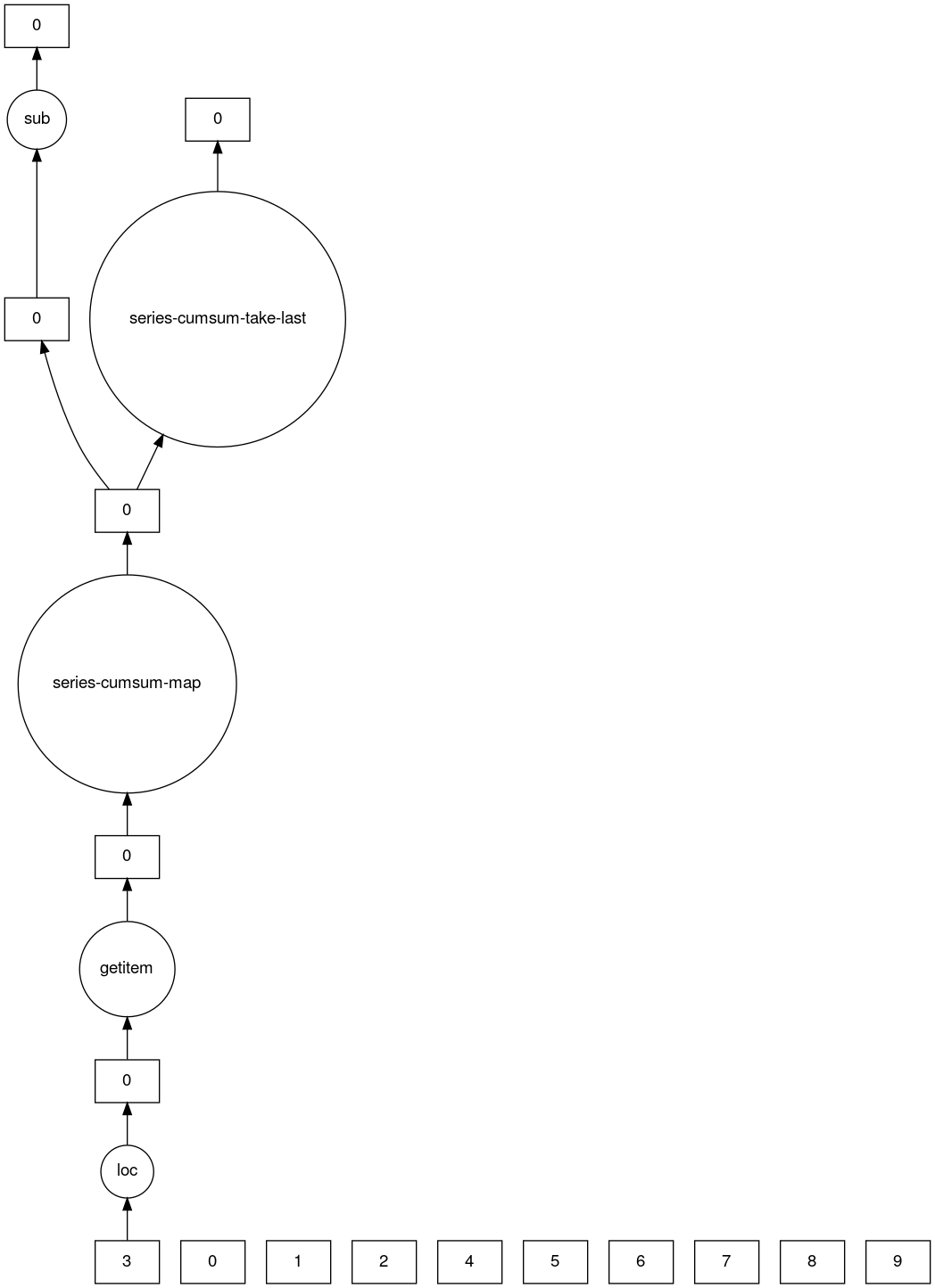
到目前为止，我们一直在设置计算并调用 compute。除了触发计算之外，我们还可以检查任务图来了解正在发生什么。


DataFrame
>>> result.dask
HighLevelGraph with 7 layers.
<dask.highlevelgraph.HighLevelGraph object at 0x7f129df7a9d0>
1. from_pandas-0b850a81e4dfe2d272df4dc718065116
2. loc-fb7ada1e5ba8f343678fdc54a36e9b3e
3. getitem-55d10498f88fc709e600e2c6054a0625
4. series-cumsum-map-131dc242aeba09a82fea94e5442f3da9
5. series-cumsum-take-last-9ebf1cce482a441d819d8199eac0f721
6. series-cumsum-d51d7003e20bd5d2f767cd554bdd5299
7. sub-fed3e4af52ad0bd9c3cc3bf800544f57

>>> result.visualize()





数组
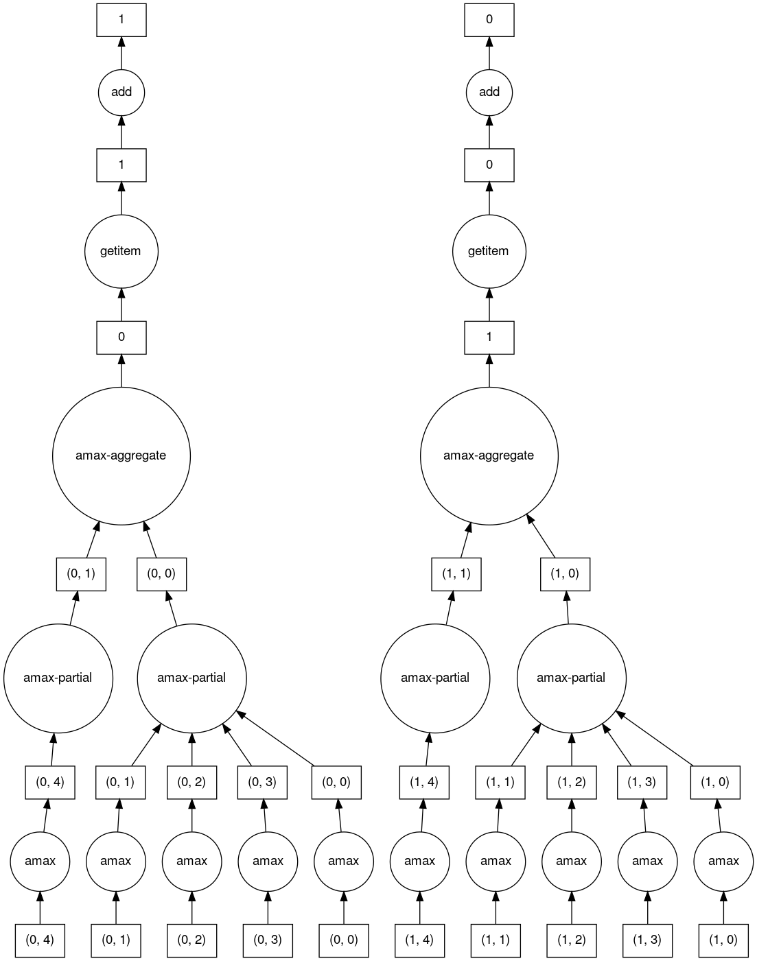
>>> b.dask
HighLevelGraph with 6 layers.
<dask.highlevelgraph.HighLevelGraph object at 0x7fd33a4aa400>
1. array-ef3148ecc2e8957c6abe629e08306680
2. amax-b9b637c165d9bf139f7b93458cd68ec3
3. amax-partial-aaf8028d4a4785f579b8d03ffc1ec615
4. amax-aggregate-07b2f92aee59691afaf1680569ee4a63
5. getitem-f9e225a2fd32b3d2f5681070d2c3d767
6. add-f54f3a929c7efca76a23d6c42cdbbe84

>>> b.visualize()





Bag
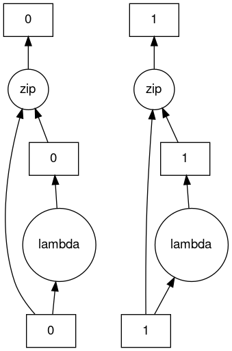
>>> c.dask
HighLevelGraph with 3 layers.
<dask.highlevelgraph.HighLevelGraph object at 0x7f96d0814fd0>
1. from_sequence-cca2a33ba6e12645a0c9bc0fd3fe6c88
2. lambda-93a7a982c4231fea874e07f71b4bcd7d
3. zip-474300792cc4f502f1c1f632d50e0272

>>> c.visualize()







低级接口¶
通常在并行化现有代码库或构建自定义算法时，会遇到可并行化但不仅仅是一个大 DataFrame 或数组的代码。


Delayed: 惰性
Dask Delayed 允许您将单个函数调用包装到惰性构建的任务图中
import dask

@dask.delayed
def inc(x):
   return x + 1

@dask.delayed
def add(x, y):
   return x + y

a = inc(1)       # no work has happened yet
b = inc(2)       # no work has happened yet
c = add(a, b)    # no work has happened yet

c = c.compute()  # This triggers all of the above computations




Futures: 即时
与到目前为止描述的接口不同，Futures 是立即求值的。函数提交后计算立即开始（请参阅 Futures）。
from dask.distributed import Client

client = Client()

def inc(x):
   return x + 1

def add(x, y):
   return x + y

a = client.submit(inc, 1)     # work starts immediately
b = client.submit(inc, 2)     # work starts immediately
c = client.submit(add, a, b)  # work starts immediately

c = c.result()                # block until work finishes, then gather result



注意
Futures 只能与分布式集群一起使用。有关更多信息，请参阅下面的部分。





调度¶
生成任务图后，执行它是调度程序的职责（请参阅 调度）。
默认情况下，对于大多数 Dask API，当您在 Dask 对象上调用 compute 时，Dask 使用您计算机上的线程池（也称为线程调度程序）并行运行计算。对于 Dask Array、Dask DataFrame 和 Dask Delayed 都是如此。例外是 Dask Bag，它默认使用多进程调度程序。
如果您想要更多控制，请使用分布式调度程序。尽管名称中包含“分布式”，但分布式调度程序在单机和多机上都运行良好。将其视为“高级调度程序”。


本地
这是设置只使用您自己计算机的集群的方法。
>>> from dask.distributed import Client
...
... client = Client()
... client
<Client: 'tcp://127.0.0.1:41703' processes=4 threads=12, memory=31.08 GiB>




远程
这是连接到已经运行的集群的方法。
>>> from dask.distributed import Client
...
... client = Client("<url-of-scheduler>")
... client
<Client: 'tcp://127.0.0.1:41703' processes=4 threads=12, memory=31.08 GiB>


设置远程集群有多种方法。有关更多信息，请参阅 如何部署 Dask 集群。


一旦您创建了客户端，任何计算都将在其指向的集群上运行。


诊断¶
使用分布式集群时，Dask 提供了一个诊断仪表盘，您可以在其中查看任务的处理过程。
>>> client.dashboard_link
'http://127.0.0.1:8787/status'


要了解有关这些图表的更多信息，请查看 仪表盘诊断。


              
            
                
 
       上一页
 Dask 安装
 
    下一页
 部署 Dask 集群


    
  © 版权所有 2014-2018，Anaconda, Inc. 和贡献者。

Dask 十分种入门

目录

Dask 十分种入门¶

创建 Dask 对象¶

索引¶

计算¶

方法¶

可视化任务图¶

低级接口¶

调度¶

诊断¶