切换导航

.rst .pdf

目录

10分钟上手Dask

这是为新用户准备的Dask简短概述。其余文档中包含更多信息。

高级集合用于生成任务图，这些任务图可以由调度器在单机或集群上执行。

我们通常按如下方式导入 Dask

>>> import numpy as np
>>> import pandas as pd

>>> import dask.dataframe as dd
>>> import dask.array as da
>>> import dask.bag as db

根据你处理的数据类型，可能不需要所有这些导入。

创建 Dask 对象

你可以通过提供现有数据并可选地包含有关分块如何构造的信息，从头开始创建 Dask 对象。

数据框 (DataFrame)

参见 Dask DataFrame。

>>> index = pd.date_range("2021-09-01", periods=2400, freq="1h")
... df = pd.DataFrame({"a": np.arange(2400), "b": list("abcaddbe" * 300)}, index=index)
... ddf = dd.from_pandas(df, npartitions=10)
... ddf
Dask DataFrame Structure:
                        a       b
npartitions=10
2021-09-01 00:00:00  int64  object
2021-09-11 00:00:00    ...     ...
...                    ...     ...
2021-11-30 00:00:00    ...     ...
2021-12-09 23:00:00    ...     ...
Dask Name: from_pandas, 10 tasks

现在我们有一个 Dask 数据框，它有2列和2400行，由10个分区组成，每个分区有240行。每个分区代表数据的一部分。

以下是 DataFrame 的一些关键属性

>>> # check the index values covered by each partition
... ddf.divisions
(Timestamp('2021-09-01 00:00:00', freq='H'),
Timestamp('2021-09-11 00:00:00', freq='H'),
Timestamp('2021-09-21 00:00:00', freq='H'),
Timestamp('2021-10-01 00:00:00', freq='H'),
Timestamp('2021-10-11 00:00:00', freq='H'),
Timestamp('2021-10-21 00:00:00', freq='H'),
Timestamp('2021-10-31 00:00:00', freq='H'),
Timestamp('2021-11-10 00:00:00', freq='H'),
Timestamp('2021-11-20 00:00:00', freq='H'),
Timestamp('2021-11-30 00:00:00', freq='H'),
Timestamp('2021-12-09 23:00:00', freq='H'))

>>> # access a particular partition
... ddf.partitions[1]
Dask DataFrame Structure:
                  a       b
npartitions=1
2021-09-11     int64  object
2021-09-21       ...     ...
Dask Name: blocks, 11 tasks

数组 (Array)

参见 数组。

import numpy as np
import dask.array as da

data = np.arange(100_000).reshape(200, 500)
a = da.from_array(data, chunks=(100, 100))
a

数组 (Array) 分块 字节数 781.25 kiB 78.12 kiB 形状 (200, 500) (100, 100) Dask 图 1个图层中的10个分块 数据类型 int64 numpy.ndarray

现在我们有一个形状为 (200, 500) 的二维数组，由10个分块组成，每个分块的形状为 (100, 100)。每个分块代表数据的一部分。

以下是 Dask 数组的一些关键属性

# inspect the chunks
a.chunks

((100, 100), (100, 100, 100, 100, 100))

# access a particular block of data
a.blocks[1, 3]

数组 (Array) 分块 字节数 78.12 kiB 78.12 kiB 形状 (100, 100) (100, 100) Dask 图 2个图层中的1个分块 数据类型 int64 numpy.ndarray

包 (Bag)

参见 包。

>>> b = db.from_sequence([1, 2, 3, 4, 5, 6, 2, 1], npartitions=2)
... b
dask.bag<from_sequence, npartitions=2>

现在我们有一个包含8个项目的序列，由2个分区组成，每个分区包含4个项目。每个分区代表数据的一部分。

索引

索引 Dask 集合的感觉就像切片 NumPy 数组或 pandas 数据框一样。

数据框 (DataFrame)

>>> ddf.b
Dask Series Structure:
npartitions=10
2021-09-01 00:00:00    object
2021-09-11 00:00:00       ...
                        ...
2021-11-30 00:00:00       ...
2021-12-09 23:00:00       ...
Name: b, dtype: object
Dask Name: getitem, 20 tasks

>>> ddf["2021-10-01": "2021-10-09 5:00"]
Dask DataFrame Structure:
                                 a       b
npartitions=1
2021-10-01 00:00:00.000000000  int64  object
2021-10-09 05:00:59.999999999    ...     ...
Dask Name: loc, 11 tasks

数组 (Array)

a[:50, 200]

数组 (Array) 分块 字节数 400 B 400 B 形状 (50,) (50,) Dask 图 2个图层中的1个分块 数据类型 int64 numpy.ndarray

包 (Bag)

Bag 是一个无序的集合，允许重复。所以它类似于列表，但不保证元素之间的顺序。由于 Bag 是无序的，因此无法对其进行索引。

计算

Dask 是惰性求值的。计算结果直到你要求时才计算出来。相反，会生成一个 Dask 任务图用于计算。

无论何时你有一个 Dask 对象并想获取结果，只需调用 compute

数据框 (DataFrame)

>>> ddf["2021-10-01": "2021-10-09 5:00"].compute()
                     a  b
2021-10-01 00:00:00  720  a
2021-10-01 01:00:00  721  b
2021-10-01 02:00:00  722  c
2021-10-01 03:00:00  723  a
2021-10-01 04:00:00  724  d
...                  ... ..
2021-10-09 01:00:00  913  b
2021-10-09 02:00:00  914  c
2021-10-09 03:00:00  915  a
2021-10-09 04:00:00  916  d
2021-10-09 05:00:00  917  d

[198 rows x 2 columns]

数组 (Array)

>>> a[:50, 200].compute()
array([  200,   700,  1200,  1700,  2200,  2700,  3200,  3700,  4200,
      4700,  5200,  5700,  6200,  6700,  7200,  7700,  8200,  8700,
      9200,  9700, 10200, 10700, 11200, 11700, 12200, 12700, 13200,
      13700, 14200, 14700, 15200, 15700, 16200, 16700, 17200, 17700,
      18200, 18700, 19200, 19700, 20200, 20700, 21200, 21700, 22200,
      22700, 23200, 23700, 24200, 24700])

包 (Bag)

>>> b.compute()
[1, 2, 3, 4, 5, 6, 2, 1]

方法

Dask 集合与现有的 numpy 和 pandas 方法匹配，因此应该感觉熟悉。调用方法来设置任务图，然后调用 compute 来获取结果。

数据框 (DataFrame)

>>> ddf.a.mean()
dd.Scalar<series-..., dtype=float64>

>>> ddf.a.mean().compute()
1199.5

>>> ddf.b.unique()
Dask Series Structure:
npartitions=1
   object
      ...
Name: b, dtype: object
Dask Name: unique-agg, 33 tasks

>>> ddf.b.unique().compute()
0    a
1    b
2    c
3    d
4    e
Name: b, dtype: object

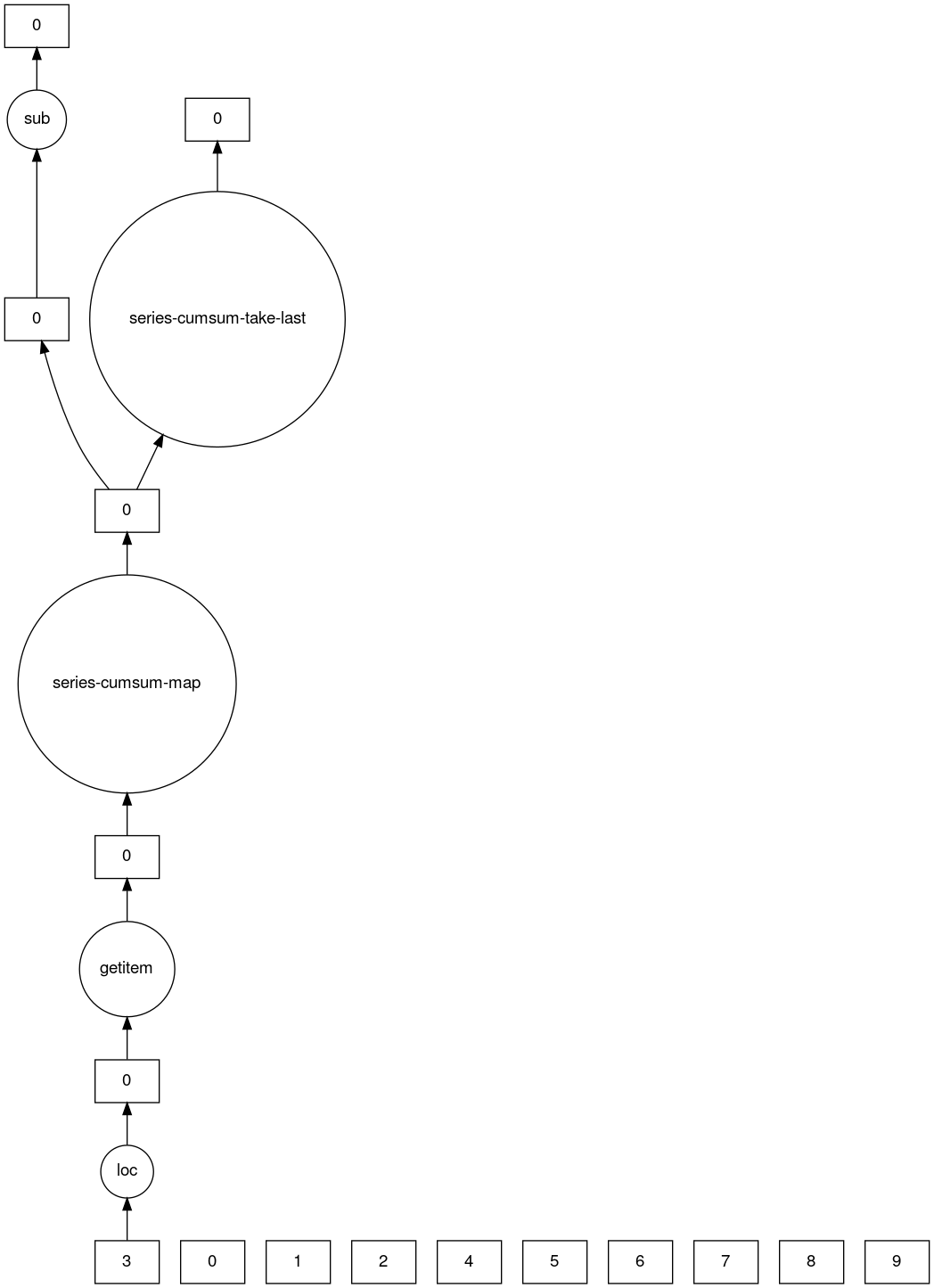
方法可以像 pandas 中一样链式调用

>>> result = ddf["2021-10-01": "2021-10-09 5:00"].a.cumsum() - 100
... result
Dask Series Structure:
npartitions=1
2021-10-01 00:00:00.000000000    int64
2021-10-09 05:00:59.999999999      ...
Name: a, dtype: int64
Dask Name: sub, 16 tasks

>>> result.compute()
2021-10-01 00:00:00       620
2021-10-01 01:00:00      1341
2021-10-01 02:00:00      2063
2021-10-01 03:00:00      2786
2021-10-01 04:00:00      3510
                        ...
2021-10-09 01:00:00    158301
2021-10-09 02:00:00    159215
2021-10-09 03:00:00    160130
2021-10-09 04:00:00    161046
2021-10-09 05:00:00    161963
Freq: H, Name: a, Length: 198, dtype: int64

数组 (Array)

>>> a.mean()
dask.array<mean_agg-aggregate, shape=(), dtype=float64, chunksize=(), chunktype=numpy.ndarray>

>>> a.mean().compute()
49999.5

>>> np.sin(a)
dask.array<sin, shape=(200, 500), dtype=float64, chunksize=(100, 100), chunktype=numpy.ndarray>

>>> np.sin(a).compute()
array([[ 0.        ,  0.84147098,  0.90929743, ...,  0.58781939,
         0.99834363,  0.49099533],
      [-0.46777181, -0.9964717 , -0.60902011, ..., -0.89796748,
      -0.85547315, -0.02646075],
      [ 0.82687954,  0.9199906 ,  0.16726654, ...,  0.99951642,
         0.51387502, -0.4442207 ],
      ...,
      [-0.99720859, -0.47596473,  0.48287891, ..., -0.76284376,
         0.13191447,  0.90539115],
      [ 0.84645538,  0.00929244, -0.83641393, ...,  0.37178568,
      -0.5802765 , -0.99883514],
      [-0.49906936,  0.45953849,  0.99564877, ...,  0.10563876,
         0.89383946,  0.86024828]])

>>> a.T
dask.array<transpose, shape=(500, 200), dtype=int64, chunksize=(100, 100), chunktype=numpy.ndarray>

>>> a.T.compute()
array([[    0,   500,  1000, ..., 98500, 99000, 99500],
      [    1,   501,  1001, ..., 98501, 99001, 99501],
      [    2,   502,  1002, ..., 98502, 99002, 99502],
      ...,
      [  497,   997,  1497, ..., 98997, 99497, 99997],
      [  498,   998,  1498, ..., 98998, 99498, 99998],
      [  499,   999,  1499, ..., 98999, 99499, 99999]])

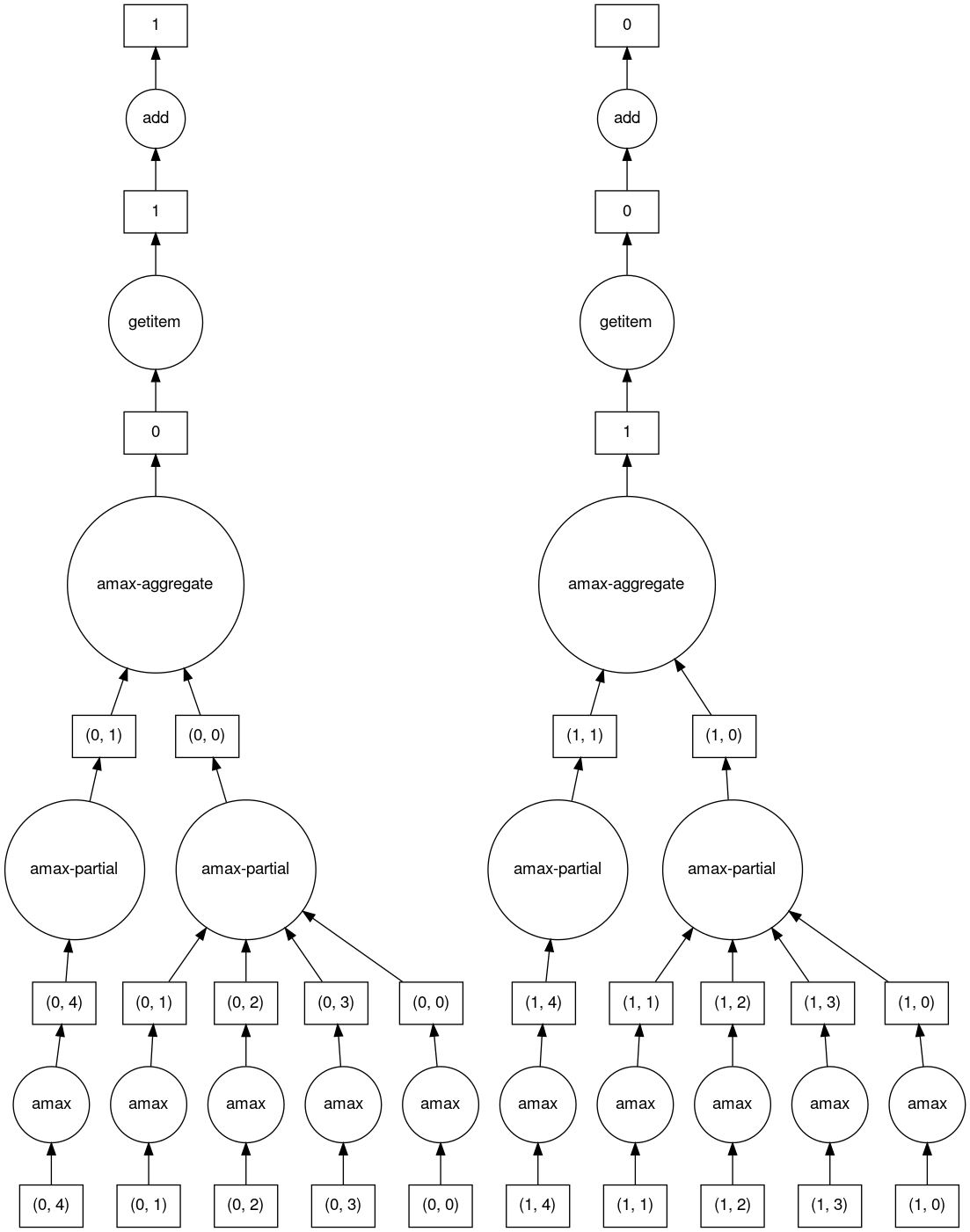
方法可以像 NumPy 中一样链式调用

>>> b = a.max(axis=1)[::-1] + 10
... b
dask.array<add, shape=(200,), dtype=int64, chunksize=(100,), chunktype=numpy.ndarray>

>>> b[:10].compute()
array([100009,  99509,  99009,  98509,  98009,  97509,  97009,  96509,
      96009,  95509])

包 (Bag)

Dask Bag 对通用 Python 对象的集合实现了诸如 map, filter, fold 和 groupby 等操作。

>>> b.filter(lambda x: x % 2)
dask.bag<filter-lambda, npartitions=2>

>>> b.filter(lambda x: x % 2).compute()
[1, 3, 5, 1]

>>> b.distinct()
dask.bag<distinct-aggregate, npartitions=1>

>>> b.distinct().compute()
[1, 2, 3, 4, 5, 6]

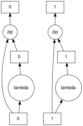
方法可以链式调用。

>>> c = db.zip(b, b.map(lambda x: x * 10))
... c
dask.bag<zip, npartitions=2>

>>> c.compute()
[(1, 10), (2, 20), (3, 30), (4, 40), (5, 50), (6, 60), (2, 20), (1, 10)]

可视化任务图

到目前为止，我们一直在设置计算并调用 compute。除了触发计算，我们还可以检查任务图以了解发生了什么。

数据框 (DataFrame)

>>> result.dask
HighLevelGraph with 7 layers.
<dask.highlevelgraph.HighLevelGraph object at 0x7f129df7a9d0>
1. from_pandas-0b850a81e4dfe2d272df4dc718065116
2. loc-fb7ada1e5ba8f343678fdc54a36e9b3e
3. getitem-55d10498f88fc709e600e2c6054a0625
4. series-cumsum-map-131dc242aeba09a82fea94e5442f3da9
5. series-cumsum-take-last-9ebf1cce482a441d819d8199eac0f721
6. series-cumsum-d51d7003e20bd5d2f767cd554bdd5299
7. sub-fed3e4af52ad0bd9c3cc3bf800544f57

>>> result.visualize()

数组 (Array)

>>> b.dask
HighLevelGraph with 6 layers.
<dask.highlevelgraph.HighLevelGraph object at 0x7fd33a4aa400>
1. array-ef3148ecc2e8957c6abe629e08306680
2. amax-b9b637c165d9bf139f7b93458cd68ec3
3. amax-partial-aaf8028d4a4785f579b8d03ffc1ec615
4. amax-aggregate-07b2f92aee59691afaf1680569ee4a63
5. getitem-f9e225a2fd32b3d2f5681070d2c3d767
6. add-f54f3a929c7efca76a23d6c42cdbbe84

>>> b.visualize()

包 (Bag)

>>> c.dask
HighLevelGraph with 3 layers.
<dask.highlevelgraph.HighLevelGraph object at 0x7f96d0814fd0>
1. from_sequence-cca2a33ba6e12645a0c9bc0fd3fe6c88
2. lambda-93a7a982c4231fea874e07f71b4bcd7d
3. zip-474300792cc4f502f1c1f632d50e0272

>>> c.visualize()

低级接口

通常，在并行化现有代码库或构建自定义算法时，你会遇到可以并行化但不仅仅是大型数据框或数组的代码。

延迟计算 (Delayed): 惰性

Dask Delayed 允许你将单个函数调用封装到延迟构造的任务图中

import dask

@dask.delayed
def inc(x):
   return x + 1

@dask.delayed
def add(x, y):
   return x + y

a = inc(1)       # no work has happened yet
b = inc(2)       # no work has happened yet
c = add(a, b)    # no work has happened yet

c = c.compute()  # This triggers all of the above computations

未来对象 (Futures): 即时

与目前为止描述的接口不同，Futures 是即时执行的。计算在函数提交后立即开始（参见 未来对象）。

from dask.distributed import Client

client = Client()

def inc(x):
   return x + 1

def add(x, y):
   return x + y

a = client.submit(inc, 1)     # work starts immediately
b = client.submit(inc, 2)     # work starts immediately
c = client.submit(add, a, b)  # work starts immediately

c = c.result()                # block until work finishes, then gather result

注意

Futures 只能用于分布式集群。有关更多信息，请参阅下一节。

调度

生成任务图后，调度器的任务就是执行它（参见 调度）。

默认情况下，对于大多数 Dask API，当你对 Dask 对象调用 compute 时，Dask 使用你计算机上的线程池（也称为线程调度器）并行运行计算。对于 Dask Array、Dask DataFrame 和 Dask Delayed 都是如此。例外是 Dask Bag，它默认使用多进程调度器。

如果你想要更多控制，请使用分布式调度器。尽管名称中包含“分布式”，但分布式调度器在单机和多机上都运行良好。把它看作是“高级调度器”。

本地

这是设置仅使用你自己的计算机的集群的方法。

>>> from dask.distributed import Client
...
... client = Client()
... client
<Client: 'tcp://127.0.0.1:41703' processes=4 threads=12, memory=31.08 GiB>

远程

这是连接到已运行的集群的方法。

>>> from dask.distributed import Client
...
... client = Client("<url-of-scheduler>")
... client
<Client: 'tcp://127.0.0.1:41703' processes=4 threads=12, memory=31.08 GiB>

有多种方法可以设置远程集群。请参考 如何部署dask集群 了解更多信息。

创建客户端后，任何计算都将在其指向的集群上运行。

诊断

使用分布式集群时，Dask 提供了一个诊断仪表盘，你可以在其中查看任务的处理情况。

>>> client.dashboard_link
'http://127.0.0.1:8787/status'

要了解有关这些图的更多信息，请查看 仪表盘诊断。

上一页

Dask 安装

下一页

部署 Dask 集群